Lab 5: Self Creation

Introduction: For lab 5, we were required to come up with our own spatial question, then use our geoprocessing skills that we have learned to answer our own question. For a while in class, I thought about what a good question would be, and a good practical one at that. While discussing with a few friends, we decided that Eau Claire could use a place to roller blade and hang out. I looked up the current location of the roller rink and realized why we never went to it, it was on the far north end of town, far away from the population who would like to use it. This brought me to my question, where within the town of Eau Claire would a roller rink be best built?

Methods: To create a map like this, I had to figure out a criteria in which to work around. I had decided I wanted the new roller rink at least 2 miles away from the current one, more would be preferred but that’s not bad. I wanted it to be placed at least within 1 mile of a school near its targeted customers. And last, it needed to be placed within the correct zoning district, as everything should be when built. Even though it would be near your customers, you can’t build a roller rink in the middle of a residential area. To begin, I plotted all schools within the state of Wisconsin, along with adding a WI base map, and a boarder around the city of Eau Claire. I removed all of the schools outside of the city with a clip, then buffered the set of schools with a 1 mile radius. I had dissolved the buffer to make a zone in which fits my school criteria. Next, I had placed the zoning classes and grouped together the main classes into 6 basic zones; Commercial, Central business, Public Properties, Industrial, Transportation, and Residential. I looked up online which zones would be used to build areas such as a roller rink or a water park (for example), and they fall under Public Properties. This now became a requirement for the new roller rink. I had used an erase with both the Public Properties zone and the already found zone which matches my school criteria, and now had a zone at least 1 mile from a school, that is a Public Property land. I had plotted the location of the current roller rink (Skate America) and followed the same process of buffering it, and erasing that zone from my current selection. The remaining zones (Highlighted in red on the map below) are areas in which match all of my criteria.

I have marked a preferred location in which to build the roller rink, as it is in a very centralized zone, matches all my criteria, and has 8 schools within a 1 mile radius of the plot. Had I further dug into the information in where I could place this, I would have looked up all available spots near my suggested area, and compared the price of rent here with others in less-preferable areas, along with the amount of expected net-profit compared a few less-preferable areas.

                Data sources: The data sources that were required for this project were the city of Eau Claire limits, all schools K-12 on to universities, the city zoning information, and a map of Wisconsin. All of this information was provided through ArcGIS online. Other sources of information would be the USGS (United States Geological Survey), but all the information I needed was collected from ArcGIS online. Again, dad I further continued this project, I could have used information collected from the US Census bureau to plot the population density of a preferable age group to the available placement land to narrow it down even more. This though, is a simple map in which to showcase my base skills.

                Results: My results are shown below. A map of the city of Eau Claire with all essential labeling, along with a data-flow model to show the geoprocesses that I have used to create this map. Restating, the map below shows the area of which could be used to build a skate arena, falling under the following criteria; Within a 1 mile limit from at last one school, in the correct zoning district, 2 miles or more away from any other roller rink, and in the city of eau Claire.

Evaluation: My overall impression of this project was positive. I enjoyed creating my own map to something that I felt was relevant to me. (I’ll be honest, working with a snail habitat a week earlier to learn how to use many of the tools was not the most exciting thing to do). If I was asked to repeat the project, I would probably have no problem working on it again. There would be a few things that I would add to it though, as mentioned above. I’d like to add the data about the expected profit value based on population of people ages 7-25 for each area to the map (probably as a graduated color map that I would add to the side). I would also like to narrow down my criteria to available land for sale or rent, so if I actually were looking for a place to build, I would not be searching in already unavailable areas.

Lab 4: Vector Analysis with ArcGIS

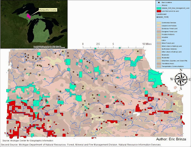
Goals and Objectives: The objectives of this lab were to create a map in which you could safely place bears, but it must fall under a few specific categories. The bears needed to be in a geological location in which *most* (at least 70%) of the other bears live, they must be placed at least 5km away from any residential area, and within the DNR management land. This lab was created to show that us as students were able to use the tools in Arc Toolbox correctly, and that we are capable of creating intricate maps with a significant value in society.

                Methods: To begin, I first plotted the points of every bear location within Marquette County Michigan. I then also added the geological map of the county. I spatially combined the bears with the geological locations to figure out which were the most prominent areas in which the bears lived. 62 out of the 68 lived within evergreen forests, forested wetlands, or mixed forest. And because this was so prominent, placing a bear in one of these three areas became one of my goals, as these were their main habitats. I then placed the streams layer to the map, (in the lab it says biologists indicated streams are important), and added a 500m buffer to the feature, as I would like to place bears close to a water source where they may drink or eat fish. I had now found a suitable bear habitats.

                The next task became to only use the area that the DNR had control over. I plotted the DNR management areas, then clipped the area that was not within the suitable habitats. This gave me the area that the DNR could place the bears within the correct habitat and under their control. Objective 5 was to make sure that area was not within 5km of a residential land or build-up. This wasn’t too hard, I just added a 5km buffer around the residential land/build-up and dissolved it. This then made a large bubble chain, in which I erased away from the suitable DNR land, leaving me only with the land that bears could live in their correct habitat, 5km away from any residential land/build-up, and under the DNR’s control. These are the areas in which bears may be placed. That actually is the result of my map as shown below.

Results: Below is the map showing land that could be used by the DNR in turquoise, and the land that could be used, but is also 5km within a residential/build-up area in red (indicating do not use). The points plotted are where all current bears have been reported as spotted, and I also added the streams to the map. Below that, you will find a dataflow model for each of the tools used in the creation of this map, and which steps they were on.

 

Sources: All sources of data were downloaded from the Michigan Center for Geographic Information
Landcover DNR Management units Streams

Lab 2

Goals and Objectives: The goal of this lab was to use the US Census Bureau to our advantage, and learn how to download information from their website and make use of it in a productive way. We were to learn how to map the data, and to get an idea to create a map ourselves. The map we created would be compared to the map that we were required to make by the first steps of the lab.

            Methods: To complete this lab, I started by going to the US Census Bureau and downloading the information required, which was the population of Wisconsin by age and locations. This information was downloaded in tables, which we could not use without a bit of touch ups. We were required to then download the shape files as well from the Census Bureau, which wasn’t much of a problem. Once these were both downloaded, we needed to change the table that we created into an actual plot-able shape file. Next, I combined the downloaded shape file and table with the information. This left me with an actual file that I could use to create a map. Mapping the data wasn’t hard, I just added it to the map then worked on its symbology layer for a while so I could create a map with the population density of Wisconsin based on the counties.

            As the lab required though, I created a second map based off of what I thought could be useful. After downloading more information and repeating the process above, I created a new map to put next to the first one, this time showing the population of males age 65 and above. I guessed that they would be more to the north before I created this, mainly because of hunting lands and cabins that people retire too. This could be very useful to find locations to place businesses that focus their sales to older men who prefer to spend their time hunting and fishing.

Results: Creating a population map that could be based off of any age, any gender, any ethnicity, or a combination of them could be insanely useful for a business to find a location to set up shop. Districts could find new locations to place schools based off of where children are in high density and far away from current learning institutions. The map below shows data from the 2010 US Census, and the information came from the US Census Bureau.

 

Geog 335 Lab 3: Introduction to GPS

Goals and Objectives: The main goal of this project was to learn how to use a Trimble Juno device to map points, lines, and polygons accurately. Along with this developed skill, learning how to transfer these points to Arc GIS to create a usable map from data in the field was another major goal of this lab.

Methods: To complete this lab, the first thing we learned how to do was use a Trimble Juno device in the field. The capabilities of this device is strong, but the speed it runs at almost counteracts its usefulness (at least it feels like it does), but it is still gets the job done. To start the lab, I had downloaded a satellite image of the area onto my Juno, along with a map of where all buildings exist/existed as of 2010. The building location was not up to date, which is why you will see a building where one does not exist on the map. I left this as reference, it could be removed easily if needed to.

 Next, I went out into the field and plotted 6 separate points, adding a label to each feature (trees x3, poles x3). Nothing too difficult there, and I continued on to plot 6 grassy areas. Three of these areas were created using point streaming, which means you can walk in any direction and it will constantly update the line that you’re creating. The other three were created point by point, at every major turn of the polygons I created, I plotted a point on the device. This makes the lines perfectly straight in the polygon. And last, I created a line across the campus footbridge. The only other piece of equipment I used would be my longboard, but that was mainly to make this lab go faster (success).

Third, moving over the data from the Juno device into a map took a bit of work. Converting files never sounds fun, but once you’ve done it enough it doesn’t take any time at all. Making the map cartographically pleasing was fun. I learned how to change the image of the points into things that better represented the objects. Instead of just different colored points for the trees and the light posts, I was able to change the trees into actual images of green trees. I also changed the light posts into pushpins. I would have created them bigger to see, but since I am working from a satellite image, I don’t think a large point to represent a single tree or lamp post would be appropriate. I also added a legend to show what every color and line represents, along with changed the grassy areas from a light green tint over my aerial picture, to an actual grassy area image. To finish it off, I placed a north aero on the map, along with a scale, and my sources (where I had got the satellite image from.

Results: For the results, I have this map of the UWEC campus to show.

GIS I Lab 1: Base Data

Goal and Background: In this lab, I am working as an intern at a company named Clear Vision Eau Claire. Clear Vision Eau Claire had just announced a partnership between local developers, and they intend to construct a new development at the confluence of the Chippewa River, and the Eau Claire River. This development, which has been named the “Confluence Project”, plans to break ground on a new community art center, along with university student housing and a commercial retail complex. All of which beginning in the year of 2014.

The goal of this project was to prepare a basic report containing all relevant information and base maps for the Confluence Project.

Methods: To do this lab, many various steps were taken for each individual map of the confluence project. To begin, all maps contained a digitized area of the proposed site for the Confluence Project, as well as an aerial map set in the background.

               The first Civil Divisions map required a layer that showed the municipality of the city of Eau Claire. To do this, I added in the data frame for civil divisions (already provided), and changed the colors to easier to see than all orange. To show the entirety of the city, I had to zoom out quite a ways, which in turn made the proposed site rather small. I then added a callbox to the proposed site.

                For the Census Boundaries map, I had added in all of the information about census boundaries into a layer, and set a clear cyan boarder around each section. To help with sorting, I added in the most recent population layer I had available (2007), and set it to 5 separate sections for an easy-to-see population grid.

               The Public Land Survey System grid was a bit easier to create. Along with the basic digitizing of the proposed site and adding in the aerials, adding the PLSS Quarter Quarter Section and changing it from a filled color to a hollow outline which shows the land easier was fairly simple.

               For the EC City Parcel Data map, I added the center lines for all roads, the parcel area for all buildings, and the water layer for each of the rivers. I edited the partial area to be hollow to show the buildings individually, and made them a color that is not to overwhelming to look at. The water I made a bit transparent to be able to see the shore and sandbars out in the rivers from the aerial layer. The center lines cover up quite a bit of space when making them large, so I kept them at a visible blue color which goes well with the lime green of the parcel area.

               When creating the Zoning layer, I had placed the zoning classes on the map, and made them transparent to be able to see them. My next step was to go into properties and configure the layers together, so there were not 15 individual residential or 9 separate commercial colors on the map. After combining the correct zones, I renamed them to their full names instead of symbols, and picked separate colors for each one. After this, I added in the center lines to the roads, and zoomed to an appropriate level for this map.

               For creating Voting Districts, I added in the provided layer, and turned amended the label section to add on numerical labels based on the voting districts. I zoomed out a bit to show the full extent of the voting district layer, and because of that, I decided to add another callbox to my map.

               After each individual map was created, I had placed them in an equally measured grid and labeled each map appropriately. I added legends for each individual map to explain what each layer meant, and sourced where my information came from at the bottom. At the end, I looked up the details within the partials online for each of the buildings within the proposed site, and  posted my findings below.

Results:

PARCEL 1

Parcel Number: 02-0357

PIN: 1822122709200042063

Street Number: 202

Street Name: EAU CLAIRE ST

Owner’s Name: Haymarket Concepts LLC

Owner’s Address: 3506 Oakwood Mall DR

Owner’s City, State, Zip: EAU CLAIRE, WI 54701

Legal Descriptions: LOT 1 AND W 1/2 OF LOT 2 BLK 58 AND A PC OF LAND BEG AT SW COR OF SAID BLK 58 THC W ON N LN OF EC ST 45 FT THC N PRLL WITH W LN OF SAID BLK 145 FT THC E PRLL WITH N LN OF SAID BLK 106 1/2 FT THC SLY PRLL WITH W LN OF SAID BLK TO N LN OF LOT 2 OF SAID BLK THC WLY ON THE N LN OF SAID BLK TO N W COR OF SAME OR LOT 1 BLK 58 THC SLY ON W LN OF SAID LOT 1 TO POB AND ALSO THE LAND BETW THE ABOVE DES LAND AND EC RIVER VILLAGE OF EC TID 8

PARCEL 2

Parcel Number: 02-0357

PIN: 1822122709200042063

Street Number: 202

Street Name: EAU CLAIRE ST

Owner’s Name: Haymarket Concepts LLC

Owner’s Address: 3506 Oakwood Mall DR

Owner’s City, State, Zip: EAU CLAIRE, WI 54701

Legal Descriptions: LOT 1 AND W 1/2 OF LOT 2 BLK 58 AND A PC OF LAND BEG AT SW COR OF SAID BLK 58 THC W ON N LN OF EC ST 45 FT THC N PRLL WITH W LN OF SAID BLK 145 FT THC E PRLL WITH N LN OF SAID BLK 106 1/2 FT THC SLY PRLL WITH W LN OF SAID BLK TO N LN OF LOT 2 OF SAID BLK THC WLY ON THE N LN OF SAID BLK TO N W COR OF SAME OR LOT 1 BLK 58 THC SLY ON W LN OF SAID LOT 1 TO POB AND ALSO THE LAND BETW THE ABOVE DES LAND AN D EC RIVER VILLAGE OF EC TID

Sources: Hemstead, Brenda. PLSS – Legal Descriptions. Retrieved from http://www.sco.wisc.edu/plss/legal-descriptions.html